Basic Syntax
The first few lines help set everything up. We create a new variable on the iris dataset so that we can make some more interesting plots. Second, we create a theme for our plots so that the labels and titles are readable.
library(ggplot2)
library(dplyr)

iris <- iris %>% group_by(Species) %>% mutate(Big.Leaf=ifelse(Petal.Length > mean(Petal.Length),'Big','Small'))

# Theme elements to make plot nicer
facet_theme <-
  theme(axis.text.x=element_text(size=12),    # Change x-axis value text-size
        axis.title.x=element_text(size=14),   # Change x-axis label text-size
        axis.text.y=element_text(size=12),    # Change y-axis value text-size
        axis.title.y=element_text(size=14),   # Change y-axis label text-size
        strip.text.x=element_text(size=14),
        strip.text.y=element_text(size=14))

curPlot <- ggplot(iris,aes(Sepal.Width,Sepal.Length))+geom_point(size=3)+facet_theme

# As Columns
curPlot+facet_grid(.~Species)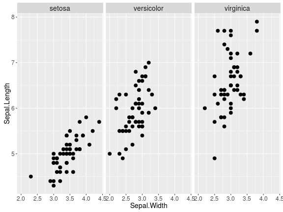
# As Rows
curPlot+facet_grid(Species~.)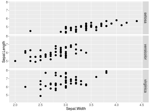
Re-ordering the panels
Simply re-order factor levels to change the order in which they’re displayed
iris$Species <- factor(iris$Species,levels=c('virginica','setosa','versicolor'))
# Remake plot with new level order
curPlot <- ggplot(iris,aes(Sepal.Width,Sepal.Length))+geom_point(size=2)+facet_theme
curPlot+facet_grid(Species~.)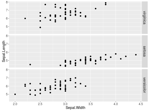
Panel By 2 Features
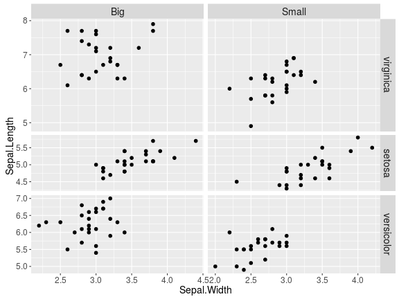
curPlot+facet_grid(Species~Big.Leaf)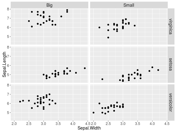
curPlot+facet_grid(Big.Leaf~Species)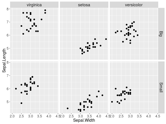
curPlot+facet_grid(Species+Big.Leaf~.)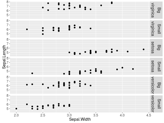
curPlot+facet_grid(.~Big.Leaf+Species)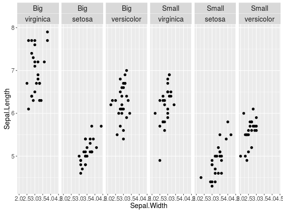
Add Marginal Panels
Single Dimension Margins
curPlot+facet_grid(Big.Leaf~Species,margins='Big.Leaf')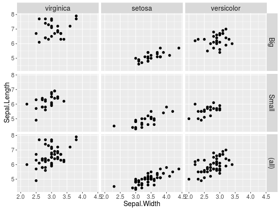
Include All Margins
curPlot+facet_grid(Big.Leaf~Species,margins=TRUE)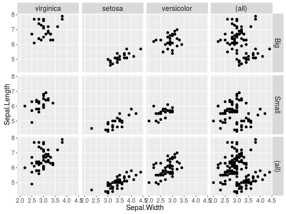
Axis Control
Normally, axes have a fixed range common to all panels and all panels are the same dimensions. We can allow the limits and the dimensions of the axes to vary freely.
curPlot+facet_grid(Species~.,scales='free')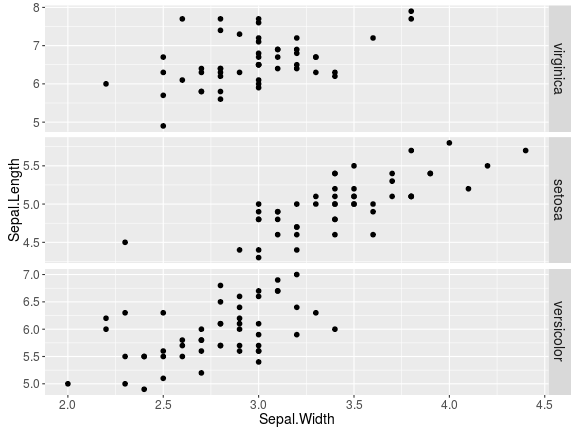
curPlot+facet_grid(Species~Big.Leaf,scales='free',space='free')