


The magrittr package offers a new operator that can help improve readability of your code, and make it easier to update and modify data wrangling code. The %>% operator has been adopted into dplyr and many of Hadley Wickham’s packages are written to be pipe-friendly.
The Problem
R code can get hard to read
sapply(iris[iris$Sepal.Length < mean(iris$Sepal.Length),-5],FUN = mean)A (Possible) Solution - the pipe %>%
- Similar to Unix pipe
| - Code can be written in the order of execution, left to right
%>%will “pipe” information from one statement to the nextx %>% fis equivalent tof(x)x %>% f(y)is equivalent tof(x,y)x %>% f %>% g %>% his equivalent toh(g(f(x)))
{magittr} provides 4 special operators
%>%- pipe operators%T>%- tee operator%$%- exposition operator%<>%- compound assignment pipe operator
What %>% is doing
The %>% is taking the output of the left-hand side and using that for
the first argument of the right-hand side, or where it finds a .
Basic Example
df <- data.frame(x1=rnorm(100),x2=rnorm(100),x3=rnorm(100))

df %>% head(1)  # same as using head(df,1)
## x1 x2 x3
## 1 0.9836479 0.4554726 -0.3232914df %>% head(.,1) # same as using head(df,1)## x1 x2 x3
## 1 0.9836479 0.4554726 -0.3232914A slightly more complicated example
library(ggplot2)
mtcars %>%
  xtabs(~gear+carb,data=.) %>%
  as.data.frame %>%
  ggplot(.,aes(x=gear,y=carb,size=Freq)) +
  geom_point()
An even more complicated example
# Generate some sample data.
df <-
  data.frame(
    Price    = 1:100 %>% sample(replace = TRUE),
    Quantity = 1:10  %>% sample(replace = TRUE),
    Type     =
      0:1 %>%
      sample(replace = TRUE) %>%
      factor(labels = c("Buy", "Sell"))
)The combination of %>% with {dplyr}
filter()group_by()summarise(),summarize()arrange()mutate()select()
sapply(iris[iris$Sepal.Length < mean(iris$Sepal.Length),-5],FUN = mean)## Sepal.Length Sepal.Width Petal.Length Petal.Width
## 5.19875 3.13375 2.46250 0.66375iris %>%
mutate(avg.length=mean(Sepal.Length)) %>%
filter(Sepal.Length<avg.length) %>%
select(-Species,-avg.length) %>%
summarise_each(funs(mean))## Sepal.Length Sepal.Width Petal.Length Petal.Width
## 1 5.19875 3.13375 2.4625 0.66375%$% The exposition operator
- Similar to
with()orattach() - Useful for functions that don’t take a data parameter
table(CO2$Treatment,CO2$Type)##
## Quebec Mississippi
## nonchilled 21 21
## chilled 21 21# with(CO2,table(Treatment,Type))
CO2 %$% table(Treatment,Type)## Type
## Treatment Quebec Mississippi
## nonchilled 21 21
## chilled 21 21%T>% The Tee Operator
- Allows a “break” in the pipe.
- Executes right-hand side of
%T>%, but will continue to pipe through to next statement
iris %>%
filter(Species != 'virginica') %>%
select(Sepal.Width,Sepal.Length) %T>%
plot %>%  # Make scatterplot and keep going
colMeans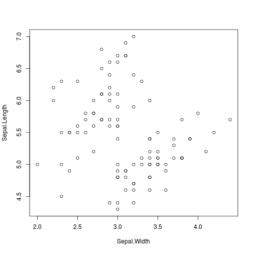
##  Sepal.Width Sepal.Length
##        3.099        5.471
%<>% The Compound Assignment Operator
- Combines a pipe and an assignment operator
- Think
i++orx+=zfrom the C family, Python, Ruby, etc.
df <- rexp(5,.5) %>% data.frame(col1=.)
df
## col1
## 1 1.9493899
## 2 0.1607936
## 3 0.1463735
## 4 2.0450395
## 5 0.3237476df %<>% arrange(col1)
df## col1
## 1 0.1463735
## 2 0.1607936
## 3 0.3237476
## 4 1.9493899
## 5 2.0450395